Update 7 march 2022: There is a new dataset available 2022-03-06, Local Time 21:22. So time comparisons can be made.
Last week, remote sensing enthusiast Sotiris Valkaniotis presented impressive maps of Landsat 8 spectral imagery in the Chernihiv Ukraine area (taken 2022-02-26 – 21.22 local time), see https://twitter.com/SotisValkan/status/1497912200857542663
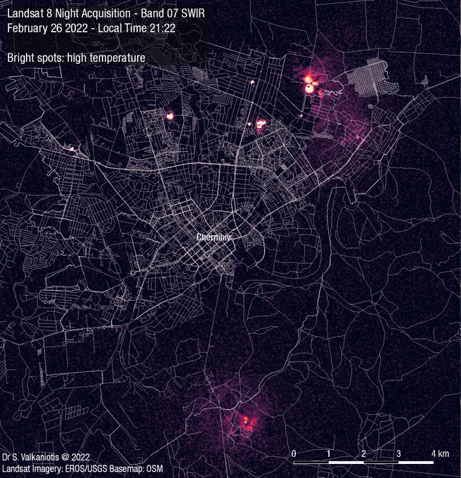
The map visualizes very high temperature in short-wave infrared band, indicating active fire fronts. 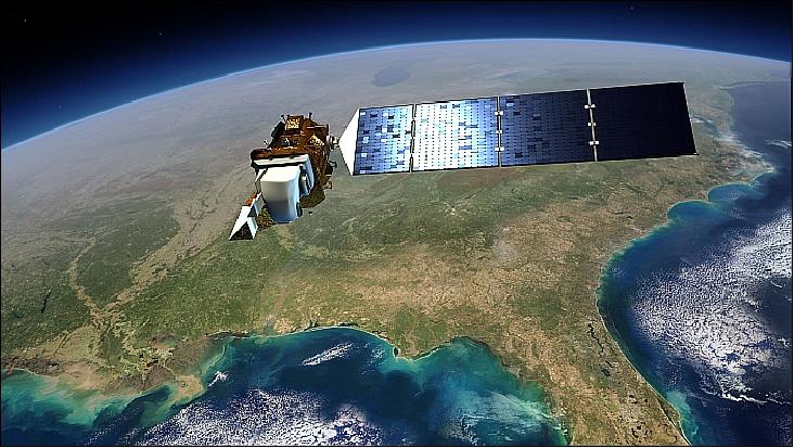
At the moment, there are 3 active Landsat 8 satellites, they observe the earth in multiple spectral bands.

Band 7 of Landsat 8 is the short wave infrared (SWIR) band (2.11-2.29 micrometer) with a resolution of 30 * 30 meter. This band is of special interest because it does work in a cloudy environment and at night.
The raw Landsat satellite images are freely available at https://earthexplorer.usgs.gov/ , to download images you need to create an account. In this blog we will investigate how to create these maps. We need to execute 3 tasks: download, process and visualize data.
Download data
To get the Landsat 8 image first go to the area of interest in https://earthexplorer.usgs.gov/, press ‘Use map’ button and select the ’data range’ containing 2022-02-26:

In the next screen, select Landsat Collection 2 Level 1, Landsat 8-9 OLI/TIRS C2 L1:

The dataset is displayed:

Click ‘Download options’, a popup appears:

Click ‘Product Options’, the various bands appear, select band 7 (B7) file (36.63MB) and download the file:

Result is the file ‘LC08_L1GT_038220_20220226_20220226_02_RT_B7.TIF’, this a GeoTIFF file (https://en.wikipedia.org/wiki/GeoTIFF – this is a TIFF containing geographical coordinates).
Process data
First get information about the image using ‘gdalinfo’:
$ gdalinfo LC08_L1GT_038220_20220226_20220226_02_RT_B7.TIF –stats
Information obtained:
– Image size: 7851 * 7941
– Projection: EPSG: 32636 (https://epsg.io/32636)
– Extent: 301485, 56084585, 537015, 5846715
– Pixel size: 30*30meter
STATISTICS_MAXIMUM=64726
STATISTICS_MEAN=5000
STATISTICS_MINIMUM=4161
So most cells have a value around 5000, with outliers almost up to 65000. We want to select only the cells with high values, so let’s filter on value = 5100 (just above the mean value). Higher value will give less cells but with higher values, lower value will give more cells.
We can filter the cells using command line tool ‘gdal_calc’ (tip use QGIS ‘OSGeo4W Shell’ on Windows to run gdal_calc):
$ gdal_calc -A LC08_L1GT_038220_20220226_20220226_02_RT_B7.TIF --outfile=calc_5100.tif --calc="A*(A>5100)" --NoDataValue=0
To avoid a blocky 30*30 meter picture we’ll resample the raster using bilinear method with gdalwarp (because a variable like heat is continuous).
$ gdalwarp -r bilinear calc_5100.tif calc_5100_bilinear.tif
Visualize data
Now we load the GeoTIFF in QGIS and style it. There are lots of options to style the layer, for example:

Result is:

With this method other Landsat 8 images can be analyzed as well, for example in Kryvyi Rih (https://twitter.com/SotisValkan/status/1497912216871395340)
